Menu
|
|
Background
A heat exchanger is a device in which energy is transferred from one fluid to another across a solid surface.
Exchanger analysis and design therefore involve both convection and conduction. Radiative transfer between the exchanger
and the environment can usually be neglected unless the exchanger is uninsulated and its external surfaces are very hot.
Two important problems in heat exchanger analysis are (1) rating existing heat exchangers and (ii) sizing
heat exchangers for a particular application. Rating involves determination of the rate of heat transfer,
the change in temperature of the two fluids, and the pressure drop across the heat exchanger. Sizing involves
selection of a specific heat exchanger from those currently available or determining the dimensions for the
design of a new heat exchanger, given the required rate of heat transfer and allowable pressure drop. The LMTD
method can be readily used when the inlet and outlet temperatures of both the hot and cold fluids are known.
When the outlet temperatures are not known, the LMTD can only be used in an iterative scheme. In this case the
 -NTU method can be used to simplify the analysis. -NTU method can be used to simplify the analysis.
Energy Considerations:
The first Law of Thermodynamics, in rate form, applied to a control volume (CV), can be expressed as

where  stands for mass-flow rate (e.g., 1bm/min or kg/min) crossing the CV boundaries, h is
specific
enthalpy (energy/mass), stands for mass-flow rate (e.g., 1bm/min or kg/min) crossing the CV boundaries, h is
specific
enthalpy (energy/mass),  surr is the rate of heat transfer from the CV to its surroundings, and surr is the rate of heat transfer from the CV to its surroundings, and
 st is the rate of change of energy stored in the CV. This simplified form of the First Law assumes
no work- producing processes, no energy generation inside the CV, and negligible kinetic and potential energy in the fluid
streams entering and leaving the CV. In steady state operation the energy residing in the CV is constant, meaning that
st =0.
If, furthermore, the boundary of the CV is adiabatic (i.e., perfectly insulated), then surr =0. Under these circumstances
Eq. (1) reduces to a simple balance of enthalpy inflow and enthalpy outflow: st is the rate of change of energy stored in the CV. This simplified form of the First Law assumes
no work- producing processes, no energy generation inside the CV, and negligible kinetic and potential energy in the fluid
streams entering and leaving the CV. In steady state operation the energy residing in the CV is constant, meaning that
st =0.
If, furthermore, the boundary of the CV is adiabatic (i.e., perfectly insulated), then surr =0. Under these circumstances
Eq. (1) reduces to a simple balance of enthalpy inflow and enthalpy outflow:

Applied to a heat exchanger with two streams passing through it, Eq. (2) can be rearranged to give:
h(hh,i-hh,o) =
c(hc,o-hc,i)
(3)
where the subscripts h and c indicate the hot and cold fluids, respectively, and i and o indicate inlet and
outlet conditions. In words, Eq. (3) says that the rate of energy loss by the hot fluid (left-hand side) equals
the rate of energy gain by the cold fluid.
Shell and Tube Heat Exchanger
Figure 1 is a schematic diagram of a shell-and-tube heat exchanger with one shell pass and one tube pass.
The cross-counterflow mode of operation is indicated.
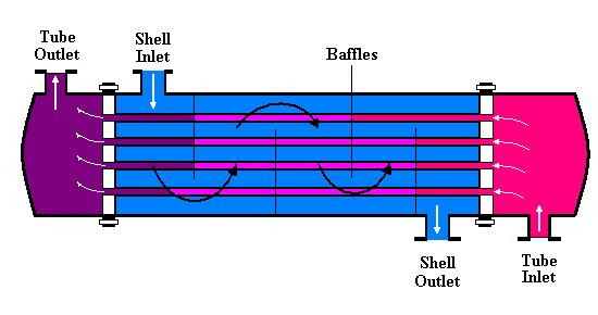
Figure 1. Shell-and-tube-heat exchanger with one shell pass and one tube pass; cross- counterflow operation.
Inside the heat exchanger the hot and cold fluid temperature distributions would have the form sketched in Fig. 2(a).

Figure 2. (a) Temperature distributions in a counterflow heat exchanger.

Figure 2. (b) Energy balance in a differential length element.
The points 1 and 2 on the x axis represent the two ends of the heat exchanger. Provided there is no energy
loss to the environment and that the exchanger has reached steady state, then dq, the rate of heat transfer from
the hot fluid, is exactly equal to the rate of heat transfer to the cold fluid in a differential length dx of the exchanger
surface. For the special case of fluids that are not changing phase and have constant specific heats
dp = -h Cp,h dTh =
- Ch dTh' &
(4)
dp = c Cp,c dTc =
Cc dTc'
(5)
where Ch and C care called the hot and cold fluid heat-capacity rates, respectively.
Integration of Eqs (4) and (5) along the heat exchanger (from 1 to 2) gives
q = Ch(Th,i-Th,o)
(6)
and
q = Cc(Tc,o-Tc,i)
(7)
1. Logarithmic Mean Temperature Difference (LMTD) Method
The differential heat-transfer rate dq across the surface area element dA can also be expressed as
dq = U TdA,
(8) TdA,
(8)
where is the local temperature difference between the hot and cold
fluids and U is the overall coefficient of heat transfer at dA. Both U and
T vary with position inside the heat exchanger (i.e., x), but by combining Eqs (4) and (5) with Eq. (8) it is
possible for a single
pass exchanger to integrate over the exchanger contact surface from inlet to out. The result of the integration is
q = AUm Tln'
(9)
where q is the total heat-transfer rate (BTU/min), A is the total internal contact area
(ft2), Um is the mean overall coefficient of heat transfer (BTU/min ft2ş F), defined as
")
and is the logarithmic mean temperature difference (LMTD), given by
")
As shown in Fig. 2(a),T1 = T h,i-Tc,o and T2 = Th,o-T c,i
for the counterflow, single pass case. Equation (9) is also applied to more complicated heat-exchanger designs
with multipass and cross- flow arrangements with a correction factor applied to the LMTD. See Ozisik (1).
As mentioned above, if both inlet and outlet temperatures are specified the LMTD can be calculated from
Eq. (11) and q from either Eq. (6) or Eq. (7). Then the product is given explicitly by Eq. (9). Further
specification of then "sizes" the heat exchanger, i.e., determines A and the dimensions of the internal flow passages.
2. -NTU Method
In cases where only the inlet temperatures of the hot and cold fluids are known, the LMTD cannot be
calculated beforehand and application of the LMTD method requires an iterative approach. The recommended
approach is the effectiveness or -NTU method. The heat-exchanger effectiveness,
, is defined by
= q/qmax,
(12)
where q is the actual rate of heat transfer from the hot to cold fluid, and qmax
represents the maximum possible rate of heat transfer, which is given by the relation
qmax = Cmin(Th,i-Tc,i)
(13)
where Cmin is the smaller of the two heat capacity rates (see above, Eqs (4) and (5).
Thus, the actual heat transfer rate can be expressed as
q = Cmin(Th,i-Tc,i)
(14)
and calculated, given the heat-exchanger effectiveness , the
mass-flow rates and specific heats of the two fluids and the inlet temperatures.
The value of depends on the heat-exchanger geometry and flow pattern
(parallel flow, counterflow, cross flow, etc.). Theoretical relations for
and graphical characteristics are given by Ozisik (1) and Incropera & DeWitt (2) for a limited selection
of heat-exchanger types. For a single pass counterflow exchanger like the one used in this exercise

where C Cmin / Cmax and N
UmA / Cmin. The dimensionless factor is known as the number of transfer units.
It is an indicator of the actual heat-transfer area or physical size of the exchanger. An experimental determination
of effectiveness is found by Cmin / Cmax and N
UmA / Cmin. The dimensionless factor is known as the number of transfer units.
It is an indicator of the actual heat-transfer area or physical size of the exchanger. An experimental determination
of effectiveness is found by

|