Chapter 3   EM Algorithm for Censored Data

 
3.1   Data Specification

For each observable vector z from a sample space , there are three possibilities depending on the observed completeness of its components: (a) all components are completely known; (b) z is only partially observed, some but not all components are completely known; (c) all components are incomplete or totally missing.

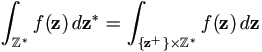
Denote the part of completely known components of z by vector z⁺ and the part of censored components by vector z^*. Without loss of generality, from now on we ignore the order of components in vector z and assume that z = (z⁺, z^*), which is indeed true when the complete and incomplete components happen to be so ordered. When z is incomplete, however, we do know that z^* belongs to an observed known set ^*. Hence, whether complete or not, z belongs to an observed known set in space , i.e. z = {z⁺} × ^* . One of the two sets {z⁺} and ^* could be empty. In case (a), z⁺= z and z^* vanishes; in case (c), z^*= z and z⁺ vanishes.

In order to uniformly handle integrals with or without partially observed data, it is convenient to make the following convention.

Definition 3.1   Suppose z is a vector with possible incomplete components z^**, and ƒ(z) is integrable, define

as the integral obtained by first plugging in values of fully observed components into the integrand, then integrating over ^* for incomplete components. If no ambiguity, denote it by

ƒ(z) dz.

(3.1)

It is obvious that: case (a) if all components of z are complete, it is just ƒ(z); and case (c) if all components of z are incomplete, it is ƒ(z) dz.

 
3.2   Likelihood Functions

Postulate a family of densities h(z|) over the full space . Now that z = (z⁺, z^*) = {z⁺} × ^* , let y = z⁺. It is easy to know that, whether complete or not, its contribution to likelihood function is proportional to g(y|) as in equation (2.1),

g(y|) = h(z|) dz*.

(3.2)

If we have a random sample with n independent observations z₁, z₂, ..., z_n, and each z_{i i}, then

g(y|) =	h(zi|) dzi,	(3.3)
ƒ(x|) =	h(zi|).	(3.4)

 
3.3   EM Algorithm with Censored Data

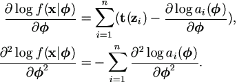
In order to maximize the likelihood in (3.3), we apply the general EM algorithm (Dempster et al., 1977) to (3.4). We first derive general equations for any distribution, and then specifically for distributions in the exponential family.

3.3.1   General Distributions

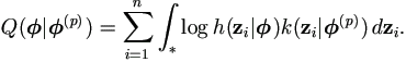
The E-step of the EM algorithm applied to (3.4) requires us to calculate (2.4),

(3.5)

Let us denote the conditional distribution of z given z and as

(3.6)

Note that if z is completely known, k(z|) = 1.

Lemma 3.1.  

(3.7)

Proof.   If z_i contains incomplete components z_i^* as in cases (b) and (c), then

If z_i is completely known as in case (a), the expectation is just itself log h(z_i|), a special case of the equation above. Since log ƒ(x|) = log h(z_i|), we can uniformly write them in a compact form as

In this very general EM case, Q (|^(p)) must be obtained for all Ω, then the M-step is achieved by choosing ^(p+1) to be a value of which maximizes Q(|^(p)).

3.3.2   Exponential Family

In case where h(z|) has exponential family form with r sufficient statistics, the integrals in (3.7) need not be computed for all , since log h(z|) is linear in the r sufficient statistics. Furthermore, Q(|^(p)) can be described via estimated sufficient statistics for a (hypothetical) complete sample. Thus the M-step of the EM algorithm reduces to ordinary maximum likelihood given the sufficient statistics from a random sample from h(z|) over the full sample space .

Specifically, suppose that h(z|) has exponential-family form

h(z|) = b(z) exp(' t(z)) /a(),

(3.8)

where denotes a r×1 vector parameter and t(x) denotes a r×1 vector of sufficient statistics. Then we have

Lemma 3.2.  

(3.9)

Proof.   This is the result of direct calculation as we know

Lemma 3.3.   The M-step is to determine ^(p+1) Ω which maximizes

- log a() + 't^(p),

where is a r×1 vector.

Proof.   Since E(log b(z_i|y, ^(p)) does not involve , the M-step is to maximize

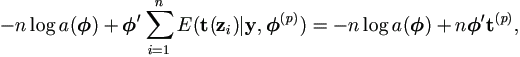
which is linear in the r components of the sufficient statistics.

Therefore we need only compute the expectations of the r components of t(z) conditional on y and given ^(p). The M-step in fact reduces to ordinary maximum likelihood given the sufficient statistics from a random sample from h(z|) over the full sample space . Based on the two lemmas, we have the EM algorithm below.

Theorem 3.1.   For exponential family with incomplete data, the EM algorithm is

E-step:	Compute
M-step:	Determine (p+1) Ω which maximizes -log a() + 't(p). For regular exponential family, it is the solution of E(t(z)|) = t(p).
Iterate the algorithm until it converges.

A Monte Carlo implementation of the EM algorithm above would be

Theorem 3.2.   For exponential family with incomplete data, the MCEM algorithm is

E-step:	For each i = 1, ..., n, draw a sample zi(1), ..., zi(m) of size m from conditional distribution k(zi|(p)). Calculate .
M-step:	Choose (p+1) to be a value of Ω which maximizes -log a() + ' (p). For regular exponential family, it is the solution of E(t(z)|) = (p).
Update the conditional distribution using (p+1), and iterate until converges.

The drawing mechanism in the Monte Carlo E-step above is a general statement. If z_i is complete, we do not need to draw any sample as then always k(z_i|)=1. In other words just let all z_i^(j) = z_i. Similarly if z_i only has some components incomplete, we draw only those incomplete components according to k(z_i|^(p)) while keep complete components intact. This remark is implied in the definition of k(z_i|) in (3.6).

3.3.3   Distributional Extension

Independent and non-identically distributed observations can be easily incorporated into the framework of this section. The extension is immediate. Under this setting, the sampling density function h(z) can be assumed different for independent observation, say h_i(z_i) for the i-th observation z_i. Then we can properly substitute h(z) by h_i(z_i) in preceding results.

First, the observed data density function in (3.3) becomes
g(y|) =	hi(zi|) dzi,	(3.10)
and the complete data density function given in (3.4) changes to
ƒ(x|) =	hi(zi|).	(3.11)

The Q-function in (3.7) turns to

(3.12)

where k_i(.) is defined with respect to h_i(.) just as k(.) in (3.6) with respect to h(.).

Exponential Family

Suppose that each h_i(z_i|) has the form (3.8) as

hi(z|) = bi(z) exp(' ti(z)) /ai(),

(3.13)

Then its Q-function in (3.9) is

(3.14)

The EM algorithm for incomplete data is then formulated as follows for independent and non-identical exponential family distributions.

E-step:	Compute
M-step:	Determine (p+1) to be a value of Ω which maximizes - log ai() + 't(p). For regular exponential family, it is the solution of E(ti(zi)|) = t(p).

 
3.4   Asymptotic Dispersion Matrix of MLE

As a maximum likelihood estimator, its asymptotic dispersion matrix is always available and given by the inverse of Fisher information matrix, which can be derived from the Hessian matrix (2.8). Now we develop the detailed asymptotic dispersion matrix for MLE with data from regular exponential family distributions.

Lemma 3.4.   Assume that z_i is from exponential family with density function h(z_i|) given by equation (3.8) as h(z_i|) = b(z_i) exp('t(z_i)) /a_i(), then

(3.15)

Proof.   As ƒ(x|) given by equation (3.4), log ƒ(x|) = log h(z_i|). Since

	then

Since t(z_i) is not related to , we have

Lemma 3.5.   Assume z_i is from regular exponential family with density h(z_i|), then

(3.16)

Proof.   This is due to the prior Lemma and the following well known equations for regular exponential family distributions,

E(t(zi)|) = log ai(),
var(t(zi)|) = log ai().

Therefore by equation (2.9) we have

Theorem 3.3.   Given a sample z_i⁽¹⁾, z_i⁽²⁾, ..., z_i^(m) for each i = 1, 2, ..., n from the distribution k(z_i|y,), the covariance matrix of can be approximated by

(3.17)

where S_i() is the sample covariance matrix from the m vectors t(z_i⁽¹⁾), ..., t(z_i^(m)) with m-1 degrees of freedom.